Continuous Improvement Tools and Techniques – Week 5 Lecture 1

Statistical Methods

During this lecture, we will discuss statistical methods in logistics management.

1. A random variable is a variable whose value is determined by the outcome of a random experiment.

2. A discrete random variable is one whose set of assumed values is countable (arises from counting).

3. A continuous random variable is one whose set of assumed values is uncountable (arises from measurement.).

We shall use:

1. A capital X for the random variable and

2. Lower case x1, x2, x3... for the values of the random variable in an experiment. These xi then represent an event that is a subset of the sample space.

The probabilities of the events are given by: P(x1), P(x2), P(x3), ...

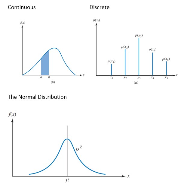
A discrete probability distribution is a table (or a formula) listing all possible values that a discrete variable can take on, together with the associated probabilities.

The function f(x) is called a probability density function for the continuous random variable X where the total area under the curve bounded by the x-axis is equal to 1

Standard Deviation of the Probability Distribution

σ=√V(X) is called the standard deviation of the probability distribution. The standard deviation is a number which describes the spread of the distribution. Small standard deviation means small spread, large standard deviation means large spread.

In the following 3 distributions, we have the same mean (μ = 4), but the standard deviation becomes bigger, meaning the spread of scores is greater.

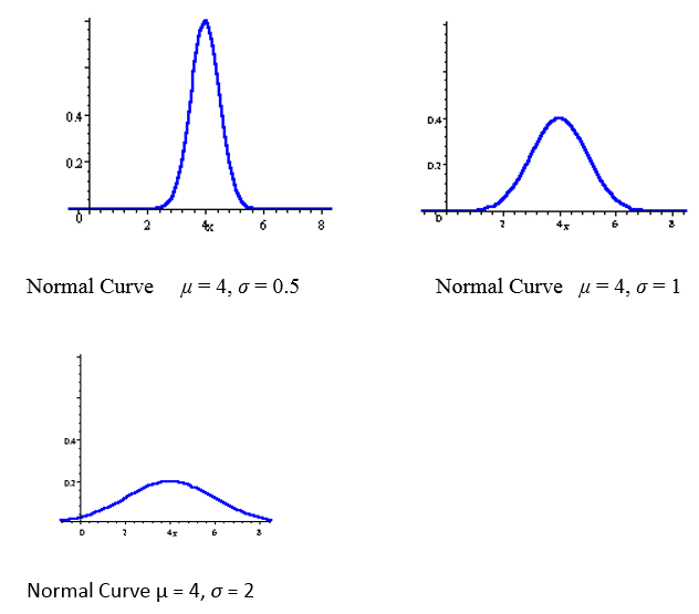
The area under each curve is 1

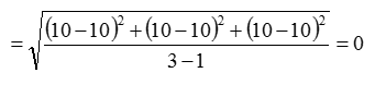
We have obtained the following data values:

10, 10, 10

The average is: 10

The standard deviation is calculated as:

Probability Distributions

A is a mathematical model that relates the value of the variable with the probability of occurrence within the population

Continuous - When the variable can be expressed on a continuous scale

Examples: Length; NPV; Weight; Strength

Discrete - When the variable can only take on certain values

Examples : Integers (0,1,2,3); Counts of items; Gender (boy / girl); Accept / Reject

Types of Distributions

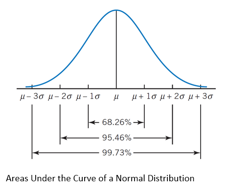
Three Zones

Zone 1: m +/- 1s

68.26% of the data is expected to be within one standard deviation of the mean

Zone 2: m +/- 2s

95.46% of the data is expected to be within two standard deviations of the mean

Zone 3: m +/- 3s

99.73% of the data is expected to be within three standard deviations of the mean

Equation for the Normal Distribution

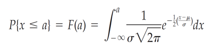
There is no closed form solution for this equation. Therefore, we take advantage of Zone rules and tables.

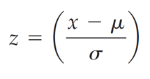
Z Value

In this equation, m is the mean, s is the standard deviation, and x is a value we would like to evaluate.

x-m calculates how far away we are from the mean

When we divide by s, we are calculating how many standard deviations we are from the mean.