Lab Assignment: Lab5 – The Fourier Series and Fourier Transform

1. Watch video entitled “Module 5 – Fourier Transform in MATLAB”

2. Perform activity 1 below for the lab assignment.

3. Include answers for Problems and include MATLAB coding along with any output plots that support solutions into a Word document entitled “Lab5_StudentID”, where your student id is substituted in the file name.

4. Upload file “Lab5_StudentID”.

IMPORTANT NOTE: You must include screenshots of MATLAB coding and MATLAB outputs in your lab submission. The screenshots MUST have the date and time stamp from Windows that appears in the lower right corner of the screen or else the lab will be worth 1%. See example below.

Activity 1:

A continuous time function is shown below in figure 1. This signal is a sinc function defined as y(t) = sinc(t). The Fourier transform of this signal is a rectangle function.

1. Use the function linspace to create a vector of time values from -5 ≤ t ≤ 5. Next, plot the function shown in figure 1 using the sinc function for y(t) = sinc(t).

2. Using Matlab and the command fft, show that the Fourier transform pair is indeed a rectangle function. Use the command fftshift to center your plot. Don't forget that the Fourier transform is complex, with both magnitude and phase. Your result should be the same as figure 2. Show both your m-file code and plot.

Matlab tip: The following commands are useful when working with the Fourier transform:

· abs gives the magnitude of a complex number (or absolute value of a real number)

· angle gives the angle of a complex number, in radians

[Note: The fft command does not give the exact transform for a continuous time signal, which we have in this case. For instance, the magnitude will not be correct. However, in order to obtain the general shape including relative magnitudes, it can be quite useful.]

3. Using the same time values, plot the continuous time function defined as y(t) = sinc(2t).

4. Plot the transform pair for this signal.

Questions:

1. What is the cause of the “ringing” seen on top of the rectangular pulse shown in figure 2?

2. In step 3 above, the sinc function gets compressed by a factor of 2, as seen by comparing the graphs in the time domain. What happened to the rectangular pulse in the frequency domain? What property does this represent?

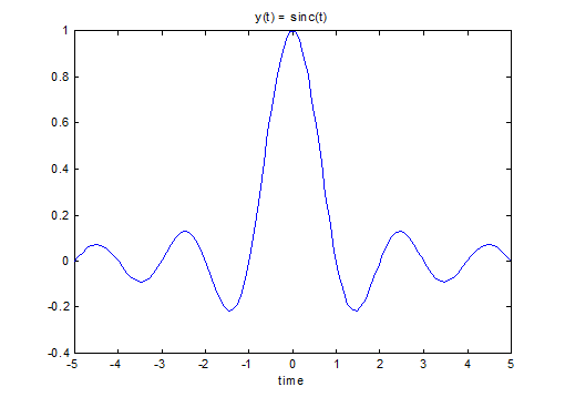
Figure 1

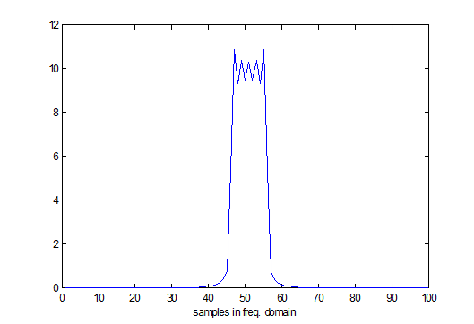
Figure 2

If you cannot view the images above, download a PDF of the Lab.  

Grading Criteria Assignments	Maximum Points
Meets or exceeds established assignment criteria	40
Demonstrates an understanding of lesson concepts	20
Clearly presents well-reasoned ideas and concepts	30
Mechanics, punctuation, sentence structure, spelling, APA formatting.	10
Total	100

Copyright 2020 // Grantham University